Program to calculate deformation due to a fault model
DC3D0 / DC3D
1 Outline of the program
DC3D0 / DC3D is the subroutine package to calculate displacement  and its space derivative
  at an arbitrary point on the surface or inside of the semi-infinite medium due to a point source (DC3D0) or a finite rectangular fault (DC3D) based on the formulation by Okada (1992) [Bull. Seism. Soc. Am., 82, 1018-1040].
From this space derivative, we can calculate strain and stress in the medium as follows.
Strain 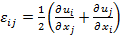
Stress 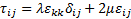 (
( are Lame constants)
【Reference】
2 Download
Fortran source code, user’s manual, and the flowchart of DC3D0/DC3D can be downloaded from the link buttons below.
For those who are interested in the mathematical background and derivation of the formula in Okada (1992), please refer to the following files.
3 How to use
DC3D0
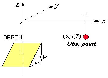
This is the subroutine to calculate displacement and its space derivative at an arbitrary point on the surface or inside of the semi-infinite medium due to a point source.
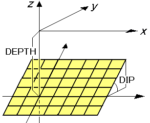
It is assumed that the medium occupies the region of z≦0, x-axis is parallel to the strike of the fault, and the location of the point source is (0, 0, -DEPTH).
CALL DC3D0 (ALPHA, X,Y,Z, DEPTH,DIP, POT1,POT2,POT3,POT4,
UX,UY,UZ, UXX,UYX,UZX, UXY,UYY,UZY, UXZ,UYZ,UZZ, IRET)
| Data | Argument | Type | Content on call | Content on return |
|---|---|---|---|---|
| Input | ALPHA | R*4 | Medium constant:=(λ+μ)/(λ+2μ) | — |
| X, Y, Z | R*4 | Location of the obs. point (Z≦0) | — | |
| DEPTH | R*4 | Depth of the point source (DEPTH≧0) | — | |
| DIP | R*4 | Dip angle of the fault (deg) | — | |
| POT1, POT2 | R*4 | Potency of left-lateral and reverse fault components(#1) | — | |
| POT3, POT4 | R*4 | Potency of tensile and explosion components(#1) | — | |
| Output | UX, UY, UZ | R*4 | — | (x,y,z) components of displacement (#2) |
| UXX,UYX,UZX | R*4 | — | x-derivative of (UX,UY,UZ)(#2) | |
| UXY,UYY,UZY | R*4 | — | y-derivative of (UX,UY,UZ) (#2) | |
| UXZ,UYZ,UZZ | R*4 | — | z-derivative of (UX,UY,UZ)(#2) | |
| IRET | I | — | Return code =0:normal =1:singular =2:positive Z was given |
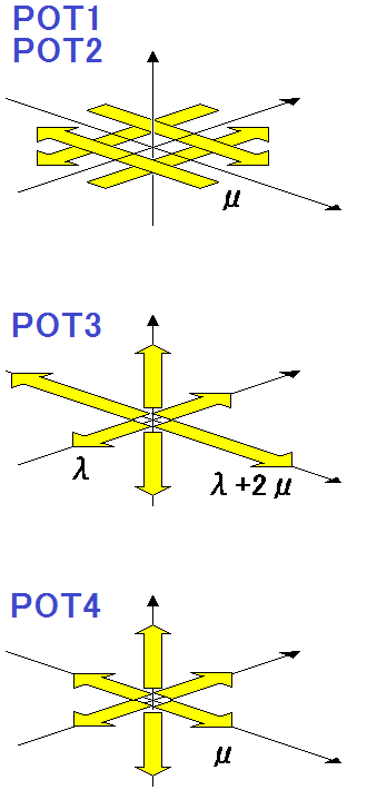
(#1)Definition of the potencies
- POT1 and POT2 : potency=(moment of double couple)/μ=LWU
- POT3 : potency=(moment of isotropic part of A-nucleus)/λ
- POT4 : potency=(moment of linear dipole)/μ
(#2)Unit of the output
- Unit for UX, UY, UZ=(unit of potency) / (unit of X, Y, Z, DEPTH)**2
- Unit for UXX….UZZ=(unit of potency) / (unit of X, Y, Z, DEPTH)**3
- So, if potency is given in the unit of cm3, and X, Y, Z, DEPTH are given in the unit of km, unit of the outputs become 1.E-10cm and 1.E-15 respectively.,
DC3D
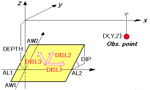
This is the subroutine to calculate displacement and its space derivative at an arbitrary point on the surface or inside of the semi-infinite medium due to a finite rectangular fault source.
It is assumed that the medium occupies the region of z≦0, x-axis is parallel to the strike of the fault, and the location of the fault origin is (0, 0, -DEPTH), from which the fault surface expands in the coordinate ranges of (AL1, AL2) and (AW1, AW2).
CALL DC3D (ALPHA, X,Y,Z, DEPTH,DIP, AL1,AL2,AW1,AW2, DISL1,DISL2,DISL3,
UX,UY,UZ, UXX,UYX,UZX, UXY,UYY,UZY, UXZ,UYZ,UZZ, IRET)
| Data | Argument | Type | Content on call | Content on return |
|---|---|---|---|---|
| Input | ALPHA | R*4 | Medium constant:=(λ+μ)/(λ+2μ) | — |
| X, Y, Z | R*4 | Location of the obs. point (Z≦0) | — | |
| DEPTH | R*4 | Depth of the fault origin (DEPTH≧0) | — | |
| DIP | R*4 | Dip angle of the fault (deg) | — | |
| AL1, AL2 | R*4 | Coordinate range of the fault in the strike direction(#1) | — | |
| AW1, AW2 | R*4 | Coordinate range of the fault in the dip direction(#1) | — | |
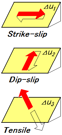
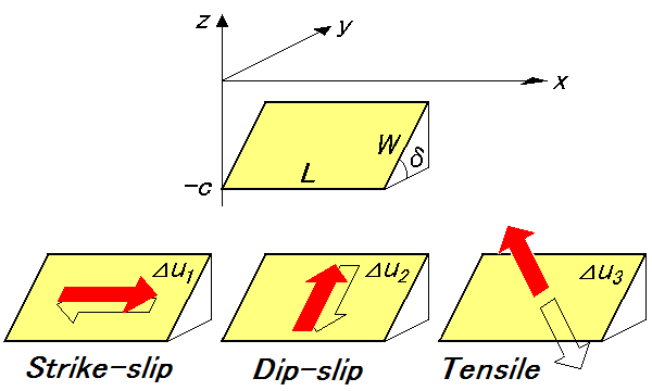
| DISL1 | R*4 | Dislocation of strike-slip component ⊿u1 | — | |
| DISL2 | R*4 | Dislocation of dip-slip component ⊿u2 | — | |
| DISL3 | R*4 | Dislocation of tensile component ⊿u3 | — | |
| Output | UX, UY, UZ | R*4 | — | (x,y,z) components of displacement(#2) |
| UXX,UYX,UZX | R*4 | — | x-derivative of (UX,UY,UZ)(#2) | |
| UXY,UYY,UZY | R*4 | — | y-derivative of (UX,UY,UZ)(#2) | |
| UXZ,UYZ,UZZ | R*4 | — | z-derivative of (UX,UY,UZ)(#2) | |
| IRET | I | — | Return code =0:normal =1:singular =2:positive Z was given |
(#1)Example to give parameters, AL1, AL2, AW1, AW2
In the case of the left figure,it should be given as AL1=0, AL2=30, AW1=-20, AW2=0, and DEPTH=10, DIP=25, DISL1=0, DISL2=50, DISL3=0
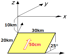
By adopting AL1, AL2, AW1, AW2, we can easily construct an inhomogeneous fault shown in the left figure.
(#2)Unit of the output
- Unit for UX, UY, UZ=(unit of DISL)
- Unit for UXX….UZZ=(unit of DISL) / (unit of X, Y, …, AW2)
- So, if dislocation is given in the unit of cm, and X, Y, Z, DEPTH, AL1, AL2, AW1, AW2 are given in the unit of km, unit of the outputs become 1.0 cm and 1.E-5 respectively.
4 Application of this program
Recent progress of space geodesy such as GPS (Global Positioning System) and SAR (Synthetic Aperture Radar) make it possible to obtain abundant and precise crustal deformation data associated to seismic and volcanic phenomena. DC3D0/DC3D can be used as a standard tool to model these phenomena as well as a powerful tool to evaluate the effect of specific seismic or volcanic event to the surrounding regions. Here, we will show several examples of such applications.
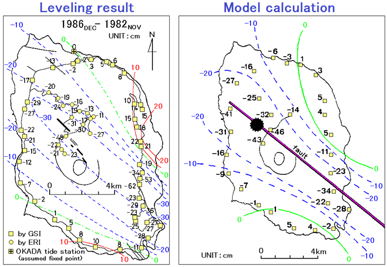
< Example 1 > 1986 Izu-Oshima eruption
Associated to the fissure eruption at the flank of Mt. Mihara in Izu-Oshima in November 1986, a party of Geographical Survey Institute carried out leveling survey surrounding the whole island and revealed the complex pattern of the vertical displacement field associated to the eruption
Theoretical formula of Okada (1985) just published was applied to this leveling data to obtain the model of magma intrusion just beneath the island with a length of 15km, a width of 10km and an opening of 2m [ Hashimoto and Tada (1988), Bull. Volc. Soc. Japan, 33, S136-S144]。
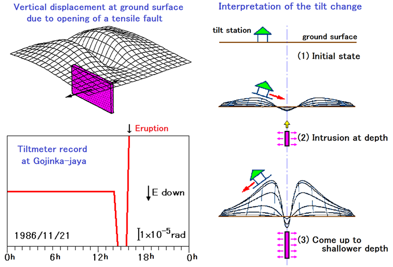
Associated to the same event, a tiltmeter installed at the Gojinka-jaya station recorded a great tilt change just before the eruption. This record was also interpreted with a model of magma intrusion to the shallower depth[Yamamoto et al. (1991), J. Phys. Earth, 39, 165-176]。
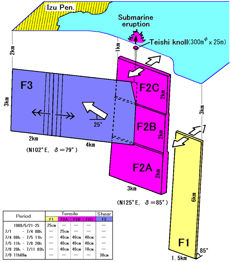
< Example 2 > 1989 Submarine eruption off Ito
Since 1978, extensive swarm activity was intermittently repeated off Ito city in the Izu Peninsula, central Japan and a small phreatomagmatic eruption took place at the ocean bottom off Ito city in July 1989.
Associated to this event, a large crustal deformation was observed in and around the eastern Izu Peninsula using tiltmeter, volume dilatationmeter, GPS and so on.
Applying the theoretical formula of Okada (1985) to these data, a quantitative model corresponding to the magma intrusion process was proposed [Okada and Yamamoto (1991), J. Geophys. Res., 96, 10361-10376]。
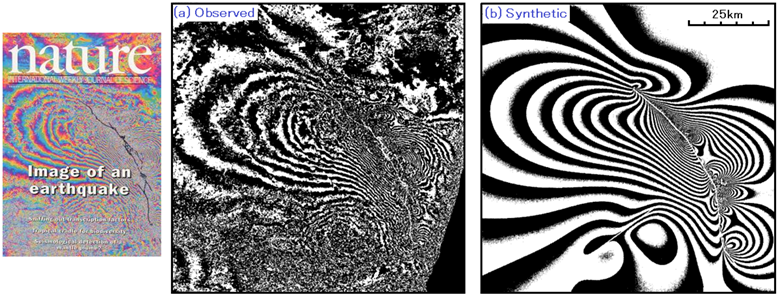
< Example 3 > 1992 Landers earthquake, 1995 Kobe earthquake
Associated to the Landers earthquake (M7.3) which took place in California, USA, in June 1992, coseismic crustal deformation was detected by SAR interferometry technique for the first time using the image by ERS-1 satellite, and the interferometric image appeared on the cover page of “Nature”.
This image was compared to the synthetic interferometric pattern calculated from the formula of Okada (1985) to estimate the fault parameters such as slip distribution of the fault [Massonnet et al. (1993), Nature, 364, 138-142]。
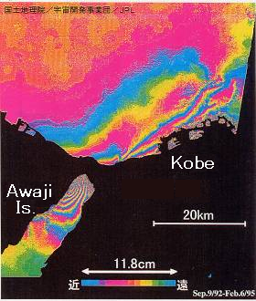
Since then, the same technique became to be applied to various seismic and volcanic events. The right figure shows an example applied to the 1995 Kobe earthquake (M7.3).
It was confirmed that the crustal deformation pattern obtained by SAR well harmonizes with the fault model [Geographical Survey Institute (2000),”Progress of Coordinating Committee for Earthquake Prediction in recent 30 years”, p.20]
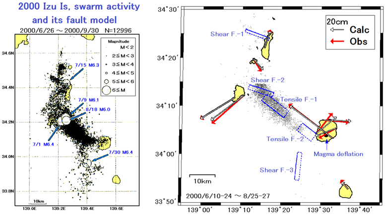
< Example 4 > 2000 Izu islands earthquake swarm
Volcanic activity at Miyakejima island which started in the end of June 2000 extended to a large scale earthquake swarm activity including the area around Niijima and Kohzujima islands accompanying a big crustal deformation. Applying the theoretical formula of Okada (1985) to these data, this activity was modeled by the combination of a number of tensile faults and shear faults [Murakami et al. (2001), Earth Monthly, 23, 791-800].
Since it was deeply concerned that this extensive swarm may trigger the hypothetical “Tokai earthquake”, the change of CFF (Coulomb Failure Function), 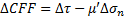 (
( : shear stress change,
  :normal stress change,
  :effective friction coefficient)was evaluated on the assumed fault of the “Tokai earthquake” using the formula of internal deformation by Okada (1992) [ Japan Meteorological Agency, 2000/9/1].
As a result, the level of stress change brought by the swarm activity was estimated to be less than a tenth of that brought by daily repeated tidal phenomenon and was judged that only little direct effect is expected.
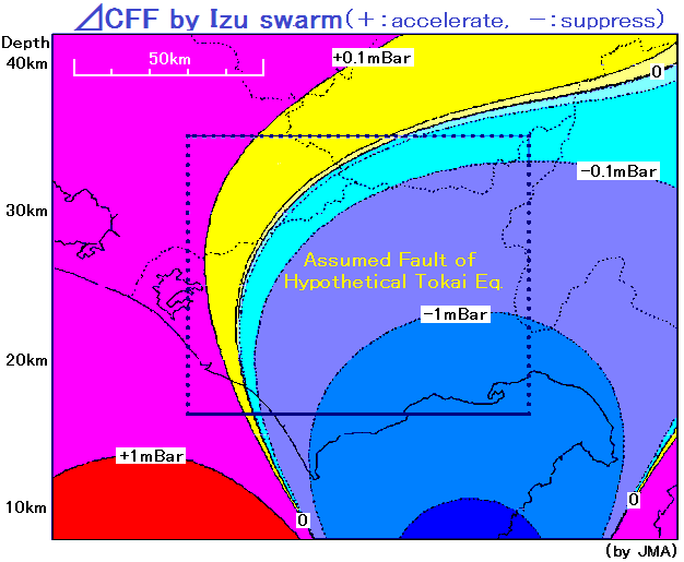
< Example 5 > 2000 western Tottori earthquake
Associated to the western Tottori earthquake (M7.3) of October 6, 2000, it was attracted the attention that a large number of aftershocks were concentrated in the area around 20km off the fault adding to the aftershocks along the fault.
The right figure shows the distribution of shear stress to generate the earthquakes similar to the main shock at the depth level of 8km in the focal region, which was calculated by the formula of internal deformation using Okada (1992) [Toda (2002), J. of Geography, 111, 233-247].
In the region of warm colors the fault becomes slippery, while it becomes hard to slip in the region of cool colors. Since the region of off-fault aftershock activity coincides to the area in which the shear stress increased, it was considered that these aftershocks were triggered by the shear stress produced by the main shock.
Thus, it becomes increasingly possible to distinguish the area easy to generate aftershocks and the area hard to generate aftershocks after the occurrence of a large earthquake.
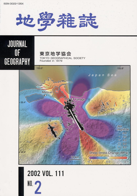
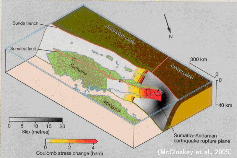
< Example 6 > 2004 Sumatra earthquake
The Sumatra earthquake (M9.1) of December 26, 2004 generated a big tsunami in the Indian Ocean causing several hundred thousand casualties. Three months later of the main shock, on March 28, 2005, a large earthquake of M8.7 again attacked the region near the Nias Island, which locates the southeastern neighbor of the focal region of the Sumatra earthquake. Right figure shows the focal regions of the both shocks after Yagi (2005).
Accidently, the possibility of the occurrence of such an induced earthquake was appointed in advance in the science magazine “Nature” published on March 17 [McCloskey et al. (2005), Nature, 434, 291].
Such a deduction was derived from the evaluation of the stress field change brought by the Sumatra earthquake using the formula to calculate internal deformation around the focal region based on Okada (1992).
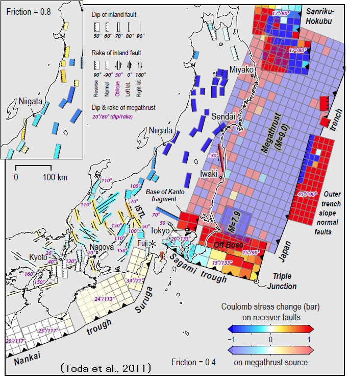
< Example 7 > 2011 East Japan earthquake
The East Japan earthquake (M9.0) of March 11, 2011, caused nearly 20 thousand casualties with a huge tsunami. This earthquake brought a large crustal deformation in the wide area of east Japan resulting extensive aftershock activities around the focal region.
It was deeply concerned that the occurrence of such a large earthquake may induce various geologic phenomena such as earthquake and volcanic eruption in the surrounding region.
The right figure shows the result of evaluation of the CFF (Coulomb Failure Function) change on the faults of inter-plate and inland earthquakes using the formula of internal deformation by Okada (1992) [Toda et al. (2011), Earth Planets Space, 63, 725-730].
In the ocean area or active faults displayed in warm colors, the occurrence of earthquake is promoted, while it is suppressed in those area displayed in cool colors.
5 Exposition
DC3D0 / DC3D are based on the papers, Okada (1985) and Okada (1992). These papers unified the shear fault which is used as a model of earthquake faulting and the tensile fault which is used as a model of magma intrusion and derived most general and compact theoretical formula to calculate deformation field on the surface(DC3D0) and the inside of the earth(DC3D).
Formulation to calculate the earth deformation due to seismic and volcanic phenomena is carried out by the following procedure.
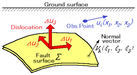
“Elasticity theory of dislocation” which considers the displacement discontinuity across a certain surface under the ground as the seismic or volcanic source was put forward by Steketee (1958) and its basic equation is presented as follows,
where,  shows the displacement vector at observation point,
  is the dislocation vector across a fault surface
  ,
,  is the normal vector to the surface ,
 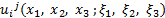 is the
  -th component of the displacement at the point
  due to a force
  in the
  -th direction placed at the point
  on the surface are elastic constants of the medium.
When we apply the above basic equation to the actual problems, there may be the following two approaches.
(1) To perform numerical integration (with brute force) using computer.
(2) To perform mathematical integration to get an analytical expression.
In principle, the approach (2) is superior than (1), because it is free from numerical errors and we can rapidly get accurate solutions.
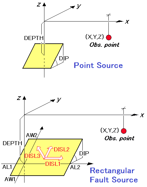
For this reason, a number of theoretical works were done by many researchers to formulate the deformation on the ground surface and the inside of the medium due to the fault of various types (right figure).
To avoid the mathematical difficulties, theoretical formula was given at first only for the simple case such as the expression for a vertical or horizontal fault in a Poisson solid (i.e.  ).
).
Thereafter the effort to get analytical solution to calculate the deformation field was continued with increasing completeness and generality of source type and fault geometry, although the majority of them were targeting shear fault as a model of earthquake source and the work targeting tensile fault as a volcanic source was rare.
In this way, there was no complete suite of closed analytical expressions which can apply to all the seismic and volcanic problems. Furthermore, not a few previous works presented too lengthy and complicated formula (sometimes ranging to several pages) even though they finally gave the same correct answer.
Okada (1985) and Okada (1992) unified the seismic and volcanic sources which had been treated separately, and gave a compact and beautiful set of closed analytical expressions which are completely general and can be applied to all the kind of fault models.
This result was picked up as “Okada model” in the glossary appeared in the Special 100th year issue (2003) of the IASPEI (International Association of Seismology and Physics of the Earth’s Interior), and widely recognized as an international standard model in this field.
DC3D0 / DC3D are utilized as a standard tool to model seismic and volcanic phenomena as well as a powerful tool to evaluate the effect of specific seismic or volcanic event to the surrounding regions. Now, Okada (1985) and Okada (1992) to which this result was submitted are counted one of the most frequently cited papers among the domestic and international scientific journals related to Seismology and Volcanology.
Also, this achievement was awarded in 2006 as The Medal with Purple Ribbon with a title, “Development of the Model for Quantitative Evaluation of Crustal Deformation”.
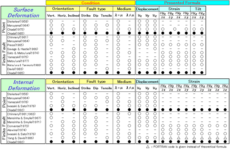
(1) Analytical formula for the surface and internal deformations so far proposed
A fault model has wide varieties in its orientation (vertical, horizontal, inclined) and fault type (strike, dip, tensile), while there are two types of the medium, Poisson solid (), and a general case ( ).
).
On the other hand, the physical quantities we need are 3 components of displacement, 4 components of strain, and 2 components of tilt for the surface deformation, whereas 3 components of displacement, and 9 components of strain for the internal deformation.
In the past, there was no complete set of formula covering all of the components listed above. Okada (1985) and Okada (1992) presented a suite of closed analytical expressions which can be applied under any combination of the fault orientation, fault type, and medium type and give all the components of the deformation (refer to the paper listed in §1 Outline of the program).
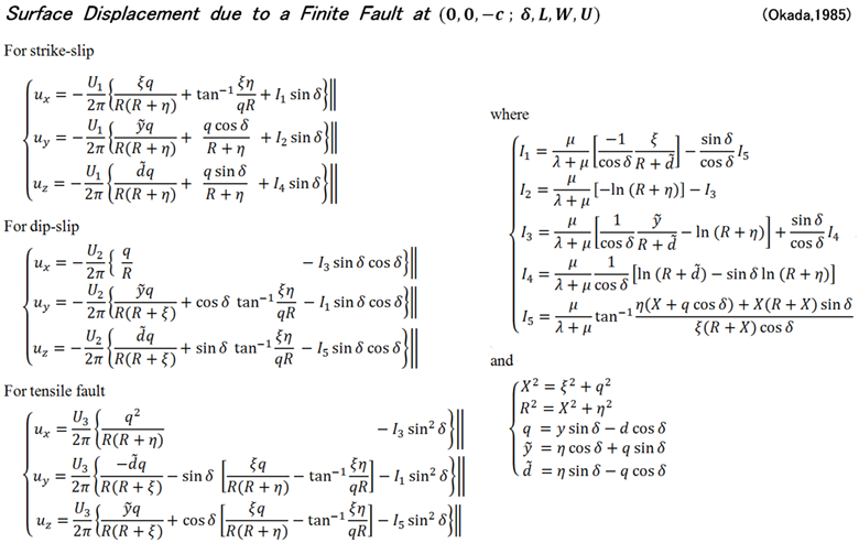
(2) Formula to calculate surface deformation due to a fault model (Okada, 1985)
The feature of this formula is its consistency among the expressions of Strike-slip, Dip-slip, and Tensile fault, as well as its compactness and beautiful style as a whole.
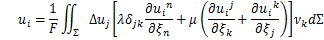
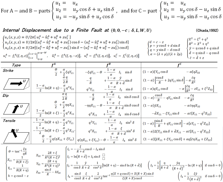
(3) Formula to calculate internal deformation due to a fault model (Okada, 1992)
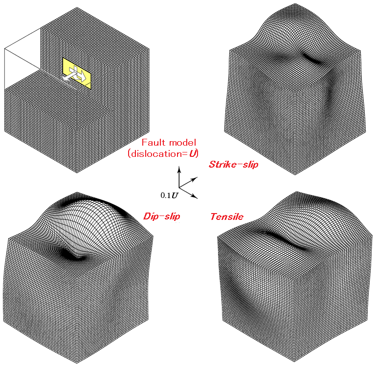
The feature of this formula is its simplicity achieved by the conversion from  , which was essentially complex, to
  using the following equation. Another feature is its compactness realized by the assembly in the form of a single table (refer to the document “Derivation of Table 6” in §2 Download).
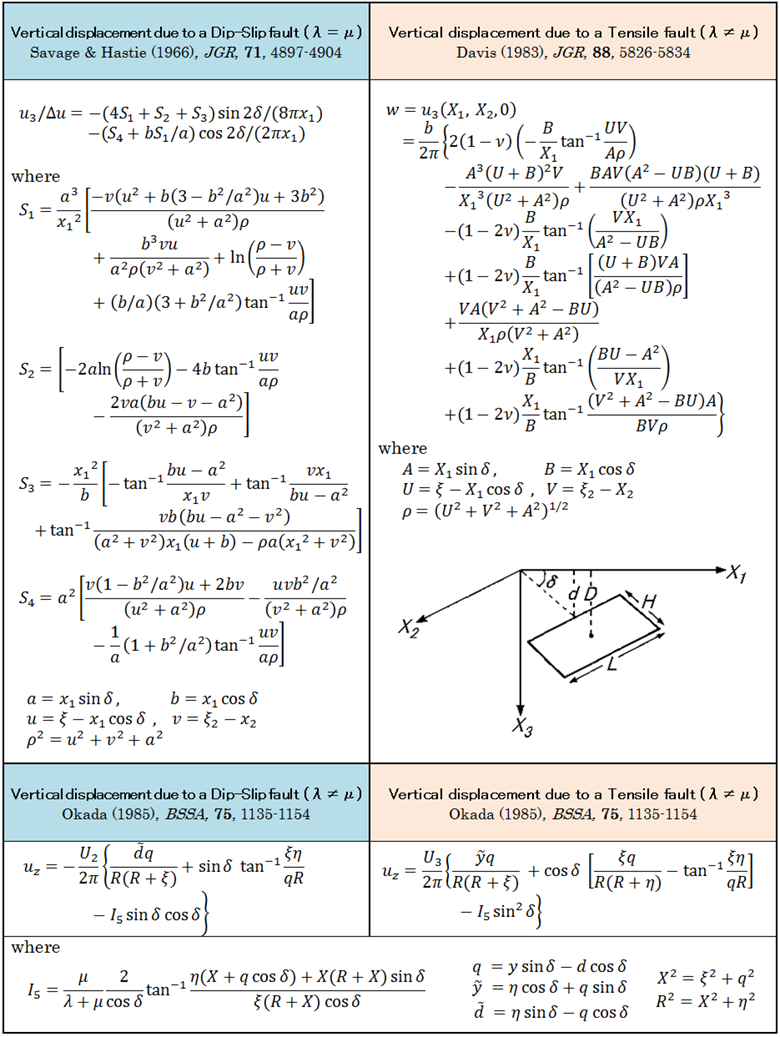
(4) Comparison to the previous work (Example 1 : Vertical displacement due to a dip-slip and a tensile fault)
Savage and Hastie (1966) proposed an equation to calculate vertical displacement  due to a dip-slip in a Poisson solid (), while Davis (1983) proposed a equation to calculate vertical displacement due to a tensile fault in a general medium ().
It was proved that these equations are mathematically identical to the formula of Okada (1985) and it was also checked that both equations give the same numerical results. It can be seen that Okada (1985)’s formula is far more compact and has consistency between the expressions of a dip-slip and a tensile fault.
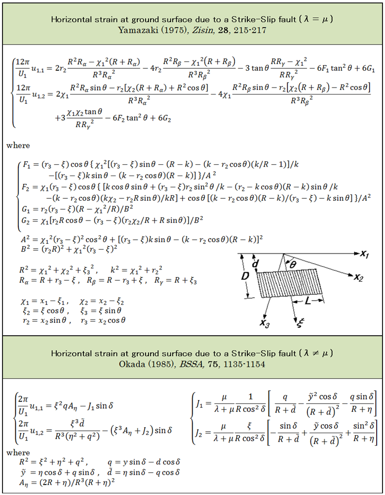
(5) Comparison to the previous work (Example 2 : Horizontal strain due to a strike-slip)
Yamazaki (1975) proposed an equation to calculate horizontal strain  due to a strike-slip in a Poisson solid (). It was also proved that these equations are mathematically identical to the formula of Okada (1985) and was again checked that both equations give the same numerical results. It can be seen that Okada (1985)’s formula is far more compact.

PDFファイルをご覧いただくには、アドビシステムズ社が配布しているAdobe Reader(無償)が必要です。Adobe Readerをインストールすることにより、PDFファイルの閲覧・印刷などが可能になります。
Adobe Readerのダウンロード